By Israr Ahmed
This article looks at three different ways in which European Cross Border Gas Capacity and Flow can be modelled in Endur. It’s also possible to combine aspects of these three models to create additional possible alternatives.
In addition we also take a look at the Position and PnL arising from modelling a gas flow from Hub to Hub.
Model 1
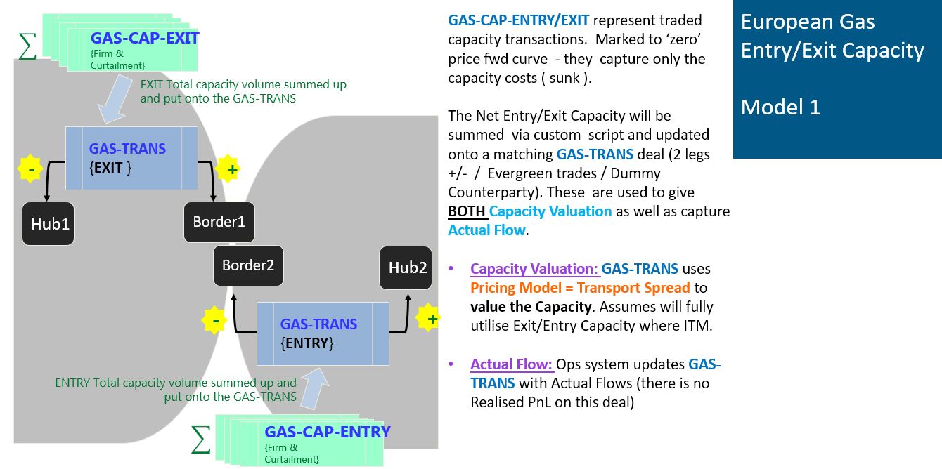
*Note that could actually also potentially have “Transport Spread Option ” on the GAS-TRANS to value to Capacity. But that would mean setting up and managing a lot of Volatilities and Correlations. Plus see the note below “A Note on Transport Spread Option v Transport Spread Model”.
Model 2
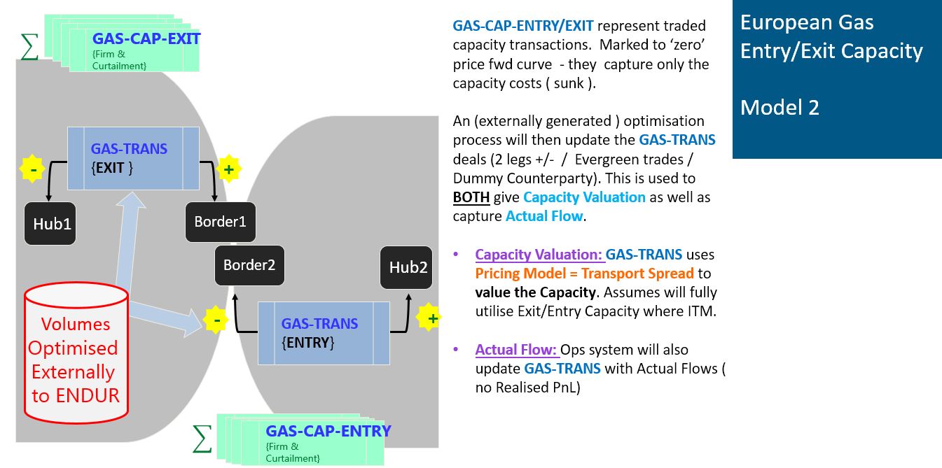
*Note that could actually also potentially have “Transport Spread Option ” on the GAS-TRANS to value to Capacity. But that would mean setting up and managing a lot of Volatilities and Correlations. Plus see the note below “A Note on Transport Spread Option v Transport Spread Model”.
Model 3
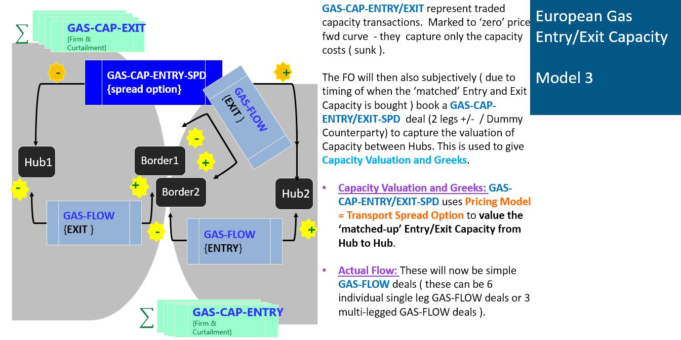
*Note that could actually also potentially have “Transport Spread” on the GAS-CAP-ENTRY-SPD to value to Capacity. See the note below “A Note on Transport Spread Option v Transport Spread Model”.
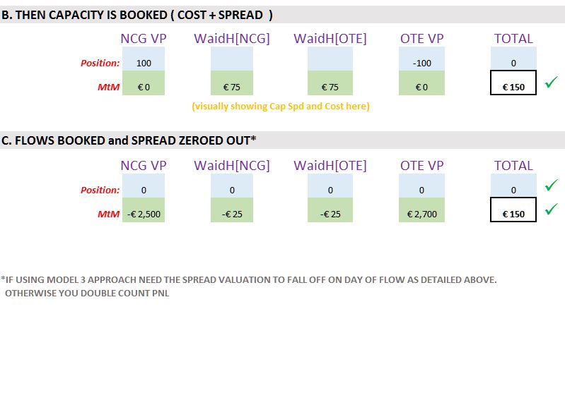
When as in Model 3 the valuation of the Spread is separate from the valuation of the Flows ( as on different deals ), there needs to be a seamless drop-off of MtM from one to the other, otherwise you double count PnL. Given that Flows are nominated on a Day Ahead basis, this means that the valuation needs to drop off the Capacity on a Day Ahead basis. However, setting the Expiry on the Spread to be 1 good business day prior ( lead days = 1d ) means that it will still show MtM on day of expiry if its in the money. Given that Flow deals would also have been booked for Day Ahead this would lead to double counting. There are two possible solutions to this.
Solution 1 : Have a customised script that runs each day and zero’s out the Day Ahead volume on the Spread Deal. A more accurate version of this would be to trigger the zeroing off when the Flow deals are booked but this could be more complex to implement.
Solution 2 : Set the Expiry on the Spread to be 2 good business days prior ( lead days = 2d ) . Whilst this ensures that on Flow nomination day the Spread is showing zero, it may lead to slight differences on the valuation Black Spread as it will generally now be a day out.
The Spread itself
One aspect to take into consideration on which Model to use, is whether the Spread is between Hub1 to Hub2 ( for which you need a Model 3 type “matching” Entry and Exit Capacity ), or a linear sum of the Spread value between Hub1->Border1 + Border2->Hub2 ( As in Model 1 and Model 2 ) . The two approaches will give different values. It is linked to whether you view the capacity valuation as separately & independently between unmatched Entry Capacity and unmatched Exit Capacity – or whether this is viewed as a matched Hub to Hub Entry/Exit Capacity.
Another aspect to consider is whether the middle GAS-TRANS / GAS-FLOW transaction ( which shows the spread between Border1 and Border2 ) is actually needed. To a certain extend this depends on whether there is any price differential between Border 1 and Border 2.
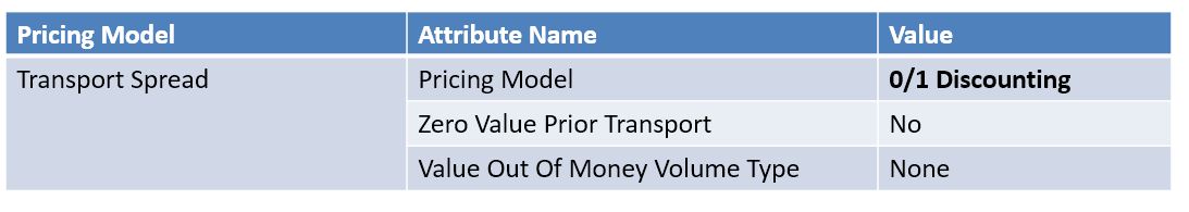
‘Transport Spread’ pricing model parameters
‘Transport Spread Option’ pricing model parameters
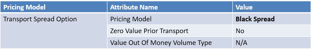
The prior value setting with the Black-Spread selected is redundant as with this model, once past the expiry date the value will be zero.
A Note on ‘Transport Spread Option’ v ‘Transport Spread’
Using “Transport Spread [ = Intrinsic ]” is simpler to implement and maintain than “Transport Spread Option [ = Black Spread ]”, as you don’t need to setup and mark Volatilities and Correlations. However because “Transport Spread ” is discontinuous at the ATM point, this results in unstable DELTA and GAMMA values when close to ATM. When it is not close to ATM it shows no GAMMA at all. So if you want the Greeks to be more stable ( and want to capture Time Value) then opt for “Transport Spread Option”. If however simplicity is a more important consideration, then opt for “Transport Spread” model.
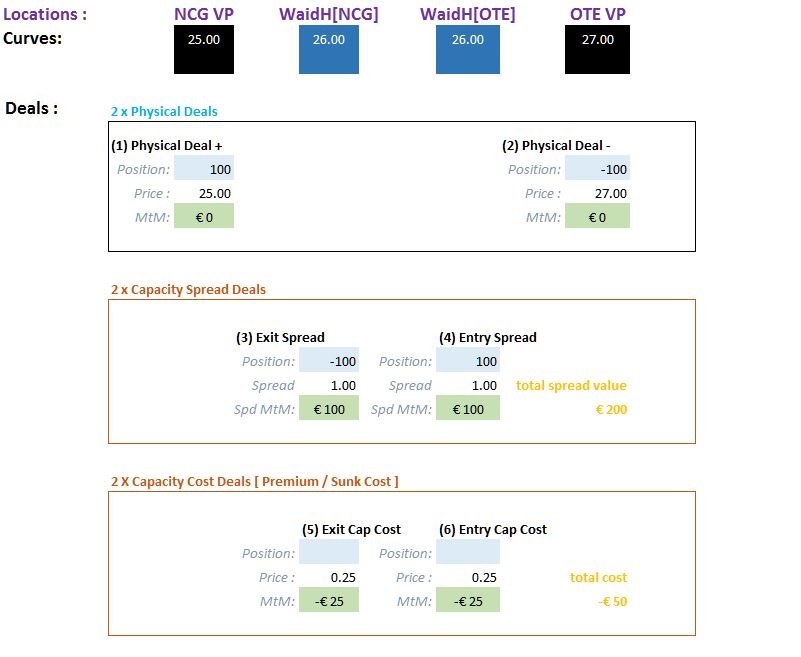
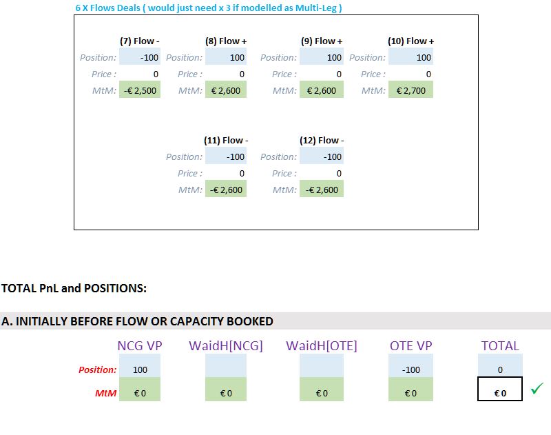
A Position and PnL visualisation of the Gas Flow process
The below example – a combination of Model 1 and Model 2 – is useful is showing the positions and PnL generated from Gas Flow process. In the example there is a EUR 2 spread between the two locations and equal notional Long/Short open position of +100 and -100. In addition there is a EUR 25 sunk capacity cost each for both the Entry and Exit Capacity.
")